ArcadeDB has had a time-series engine for a while, and it shows up in our release notes far more often than in our guides. That is an odd imbalance for something that ships columnar compression, a PromQL evaluator and a Prometheus remote-storage endpoint, so here is the guide. It covers how the engine works, what each way of getting data in costs, and the handful of behaviours that surprise people. I ran every query and request below against ArcadeDB 26.10.2.
The short version. You define a type with a timestamp, some tags and some fields. You write into it over InfluxDB line protocol, Prometheus remote_write, gRPC, SQL, or the embedded Java API. You read it back with SQL and a set of ts.* functions, with PromQL, or through Grafana. It is the same database and the same transaction that holds your graphs and documents.
If you already run time series on ArcadeDB, upgrade to 26.10.2. It fixed retention resurrecting blocks it had just dropped, COMPACT TIMESERIES TYPE racing a retention pass, and a PRECISION SECOND type losing every sample at the first retention run. The 26.10.2 release notes have the full list.
Defining a series
CREATE TIMESERIES TYPE SensorReading
  TIMESTAMP ts
  TAGS (sensor_id STRING, location STRING)
  FIELDS (
    temperature DOUBLE,
    humidity DOUBLE,
    pressure DOUBLE
  )
  SHARDS 8
  RETENTION 90 DAYS
  COMPACTION_INTERVAL 1 HOURS
Everything after FIELDS is optional; the minimal form is a timestamp, one tag and one field.
The distinction that matters is tags versus fields. Tags are low-cardinality indexed dimensions, the things you filter and group by: sensor id, host, region. Fields are the high-cardinality measurements. Getting this backwards, putting a request id in a tag, is the classic way to make a time-series database unhappy, and it is a modelling decision you cannot cheaply reverse later.
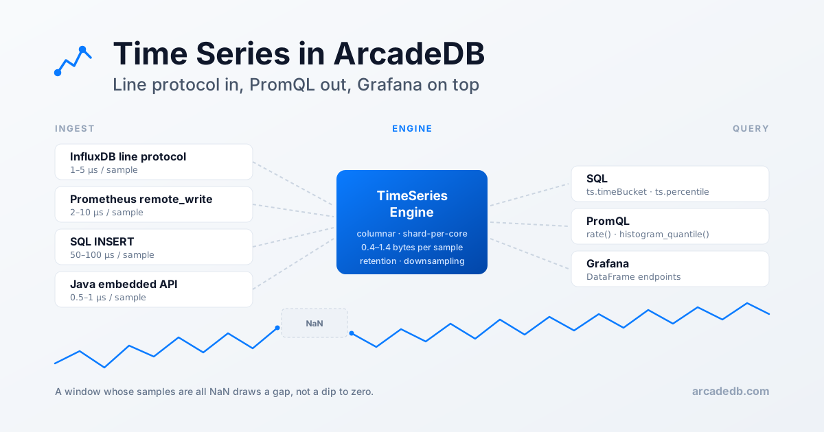
Storage is columnar, with a different compression scheme per column type: Gorilla for floats, delta-of-delta for timestamps, Simple-8b for integers, dictionary for tags. That lands between 0.4 and 1.4 bytes per sample. Writes are shard-per-core and lock-free, which is what SHARDS is tuning.
Retention and downsampling are declarative. There is no cron job to write:
ALTER TIMESERIES TYPE SensorReading
  ADD DOWNSAMPLING POLICY
    AFTER 7 DAYS GRANULARITY 1 MINUTES
    AFTER 30 DAYS GRANULARITY 1 HOURS
On a cluster, the downsampling policy replicates to followers as of 26.10.2; before that it was saved on the leader only.
Getting data in
Four classic paths, and the throughput difference between them is large enough to be the whole decision. The figures are the per-sample costs from the documentation, so treat them as orders of magnitude:
| Method | Per sample | Overhead | Use it for |
|---|---|---|---|
| Java embedded API | ~0.5 to 1 µs | none | in-process applications |
| InfluxDB line protocol | ~1 to 5 µs | text parsing | remote ingestion, Telegraf |
Prometheus remote_write |
~2 to 10 µs | Protobuf + Snappy | existing Prometheus setups |
SQL INSERT |
~50 to 100 µs | SQL parse and plan | ad-hoc and small batches |
SQL insert is fifty to a hundred times more expensive per sample than line protocol, for the ordinary reason that it parses and plans a statement per batch. Use it when it is convenient and the volume is small. 26.10.1 added a fifth path, a gRPC time-series API, for clients that already talk to ArcadeDB over gRPC.
Line protocol is the one to reach for remotely, and it is a plain HTTP POST:
curl -X POST "http://localhost:2480/api/v1/ts/mydb/write?precision=ns" \
  -u root:password \
  -H "Content-Type: text/plain" \
  --data-binary 'SensorReading,sensor_id=sensor-A,location=building-1 temperature=22.5,humidity=65.0 1791849600000000000
SensorReading,sensor_id=sensor-B,location=building-2 temperature=19.1 1791849600000000000'
The measurement name has to match the type name, and the type has to exist: a write to an unknown measurement is refused with a 400 that names it. Because this is the InfluxDB format, anything that already emits it, Telegraf and the Grafana Agent included, points at ArcadeDB with a URL change.
For an existing Prometheus deployment, ArcadeDB is a remote-storage backend:
# prometheus.yml
remote_write:
  - url: "http://localhost:2480/api/v1/ts/mydb/prom/write"
    basic_auth:
      username: root
      password: password
Each metric becomes a type named after it, and labels become tag columns, converted to the column’s declared type as of 26.10.2. remote_read is implemented too, so the data is queryable from the Prometheus side as well as from ArcadeDB’s own. ArcadeDB speaks remote write 1.0; a 2.0 body is answered with 415, so leave Prometheus on the default protocol.
Getting data out
SQL, with time-series functions
Ordinary SELECT works, and range conditions on the timestamp column push down into the storage engine:
SELECT ts.timeBucket('1h', ts) AS hour,
       sensor_id,
       avg(temperature) AS avg_temp,
       max(temperature) AS max_temp,
       ts.percentile(temperature, 0.99) AS p99
FROM SensorReading
WHERE ts BETWEEN '2026-10-13' AND '2026-10-14'
GROUP BY hour, sensor_id
ORDER BY hour
There is a full ts.* family beyond bucketing: rate with optional Prometheus-style counter-reset detection, delta, movingAvg, interpolate for gap filling with zero, previous, or linear methods, correlate for Pearson correlation between two fields, percentile, and the window functions lag, lead, rowNumber and rank.
Buckets are counted from the Unix epoch, which was a Thursday, so a 1w bucket starts on Thursday at 00:00 UTC unless you say otherwise. Since 26.10.1 ts.timeBucket takes an origin as a third argument, which gives you Monday weeks or local-midnight days:
SELECT ts.timeBucket('1w', ts, '2026-10-26') AS week, avg(temperature) AS avg_temp
FROM SensorReading
GROUP BY week
One naming trap, before it costs you ten minutes: bucket is a reserved word in ArcadeDB SQL, because buckets are a core storage concept. AS bucket fails to parse. Alias it to hour, week, tbucket, anything else.
PromQL
ArcadeDB has its own PromQL parser and evaluator, exposed on Prometheus-compatible HTTP endpoints:
GET /api/v1/ts/mydb/prom/api/v1/query?query=avg(cpu_usage{host="srv1"})&time=1700000000
GET /api/v1/ts/mydb/prom/api/v1/query_range?query=rate(http_requests_total[5m])&start=...&end=...&step=60
Plus the label-discovery endpoints (/labels, /label/{name}/values, /series) that Grafana’s query builder uses for autocomplete. /series requires a match[] selector, as it does in Prometheus.
Coverage is broad: regex label matchers, sum/min/max/avg/count/topk/bottomk/quantile with by and without, the whole rate family, the _over_time functions, histogram_quantile, the math and label functions, and the full operator set including and, or, unless and, since 26.10.2, the bool comparison modifier (a > bool 1).
You can also call it from SQL, which is more useful than it sounds when you want a PromQL expression as one column of an otherwise relational result:
RETURN promql('cpu_usage{host="srv1"}', 1700000000000)
The evaluator is strict in the same places Prometheus is. A non-numeric or out-of-range start, end, step or time is refused with 400 bad_data before the query runs, and since 26.10.2 so are the expressions Prometheus itself rejects: a comparison between two scalars without bool, a set operator with a scalar operand, a range query whose result is a range vector. If a dashboard query broke on upgrade, run it against Prometheus; it almost certainly fails there too.
Grafana
The Grafana path is the DataFrame-compatible endpoints under /api/v1/ts/mydb/grafana/ plus the Grafana plugin we shipped earlier this year. There is also a simplified JSON query endpoint that is easier to drive from application code than raw SQL:
POST /api/v1/ts/mydb/query
{
  "type": "SensorReading",
  "from": 1791849600000,
  "to": 1791936000000,
  "tags": { "sensor_id": "sensor-A" },
  "aggregation": {
    "bucketInterval": 3600000,
    "requests": [
      { "field": "temperature", "type": "AVG" },
      { "field": "temperature", "type": "MAX" }
    ]
  }
}
from, to and bucketInterval are epoch milliseconds, and a tag or field name the type does not have is refused with 400 rather than ignored. Drop aggregation and list the columns in fields for raw points. For a quick look without any of this, Studio has had a Chart tab for query results since 26.10.1.
Four things to know before you rely on it
These are the four I would tell a colleague before they put a production dashboard on top of this. All four are deliberate.
Timestamps are milliseconds
Whatever precision you write with, ArcadeDB stores, retains and queries time-series timestamps in milliseconds. The precision parameter on the line protocol endpoint tells the server how to read your timestamps, and nanosecond input is converted on the way in. Declaring the type itself as anything else is refused:
TimeSeries timestamp precision 'NANOSECOND' is not supported: timestamps are stored,
ingested, retained and queried in milliseconds, so only MILLISECOND (the default) can be declared
If you are migrating from a store that kept nanoseconds and you have two samples in the same millisecond, they now share a timestamp. Older versions accepted PRECISION NANOSECOND and PRECISION SECOND; neither worked properly, which is why 26.10.2 stopped accepting them.
Writes are strict
Since 26.10.2 the write paths refuse what they cannot store faithfully, instead of storing it wrong. A line with a field the type does not declare is dropped and reported:
{"error":"partial write: undeclared tag/field key(s): SensorReading.voltage (field) ...",
 "written":0, "dropped":1, "undeclaredKeys":["SensorReading.voltage (field)"]}
The same goes for an empty tag value, a quoted datetime in a typed column, and a value the column cannot hold. The response says how many lines were written and dropped, and which keys or line numbers were at fault, so check it rather than the status code alone.
This catches people whose Telegraf configuration sends more fields than the type declares. Before 26.10.2 the extra fields were silently discarded. Either declare them, or set arcadedb.timeSeriesUndeclaredKeys=ignore to get the old lenient behaviour for schema-less producers.
NaN means missing
A NaN sample means “no measurement here”, not zero. Every aggregation skips it: MIN, MAX, SUM and AVG are computed over the real samples in the window and ignore the rest. A window where every sample is NaN has no value at all, and over SQL, REST and Grafana that comes back as null, since JSON has no NaN literal. A Grafana panel therefore draws a gap for that bucket instead of a dip to zero. A real Infinity is a measurement and comes back as one.
Getting here took two releases, which matters if you run an older build. Before 26.9.1 an all-NaN window returned internal placeholders, 1.7976931348623157E308 from multi-column aggregation and +Inf/-Inf from PromQL’s min_over_time and max_over_time, and they looked like real measurements. If your dashboards show unexplained spikes to around 1.8e308, that is where they come from. Before 26.10.1 a single NaN made SUM and AVG of the whole window NaN.
PromQL is the exception to the null rule. Like Prometheus, its endpoints return a raw NaN sample as the string "NaN", so a series whose newest sample is missing still shows up in an instant query, with "NaN" as its value.
A time-series INSERT returns a record with no RID
Time-series points are not addressable records, so a SQL INSERT into a time-series type returns the row it wrote with no @rid. Client code that expects every inserted record to carry one, as most ORM-style wrappers do, will need to cope with its absence. The data is committed either way. It is also one more reason to use line protocol for anything at volume.
Where this fits
A dedicated time-series database will probably beat ArcadeDB on a pure ingest benchmark. The reason to keep your metrics here anyway is that a timestamp is rarely the only question you have about an event.
Time series tells you when a thing happened. The graph in the same database tells you what it was connected to. If a latency spike on one service and an error burst on another are related, the relationship is a traversal, and it is a traversal over data you did not have to export anywhere to run it against. Our fraud detection walkthrough does exactly this: transfers stream into a time-series type for the bucketed velocity checks, while the ring detection runs over the graph next to it. The same argument is behind our real-time analytics page, which covers the IoT and monitoring side in more depth.
The engine, the endpoints, and every function above are in the open-source build under Apache 2.0. There is no metrics tier.